Proof of the Theorem
We start by first treating the case where the contact manifold is \(\mathbb{R}^3\) equipped with the standard contact structure, that is, we aim to prove the following:
Proposition 2.1. Let \(\upsilon\in C^0([0,2\pi],\mathbb{R}^3)\). For every \(\varepsilon>0\) there exists a Legendrian curve \(\eta\in C^\infty([0,2\pi],\mathbb{R}^3)\) such that \(\|\upsilon-\eta\|_{C^0([0,2\pi])}\leqslant\varepsilon\).
Remark 3. Here, as usual, \(\|\gamma\|_{C^0(I)}\coloneqq \sup_{t\in I}|\gamma(t)|\) and \(\|\gamma\|_{C^1(I)}\coloneqq \|\gamma\|_{C^0(I)}+\|\mathrm{d}\gamma\|_{C^0(I)}\).
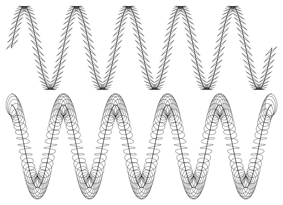
Let the curve we wish to approximate be given by \((x,y,z)\in C^\infty([0,2\pi],\mathbb{R}^3)\). The regularity is no restriction due to a standard approximation argument using convolution. Let \(\eta=(a,b,c) \in C^\infty([0,2\pi],\mathbb{R}^3)\) denote the approximating Legendrian curve. For every choice of smooth functions \((a,c) \in C^\infty([0,2\pi],\mathbb{R}^2)\) satisfying \(\dot{a}\neq 0\), we obtain a Legendrian curve by defining \(b=\dot{c}/\dot{a}\). Therefore, if \((\dot{a}(t),\dot{c}(t))\) lies in the set \[\mathcal R_{t,\varepsilon}\coloneqq\left\{(u,v)\in\mathbb{R}^2,|v-y(t)u|\leqslant \varepsilon \min\{|u|,|u|^2\}\right\},\] for every \(t \in [0,2\pi]\), then \(\|b-y\|_{C^{0}([0,2\pi])}\leqslant \varepsilon\). This condition can be achieved by defining \[(a(t),c(t)):=(x(0),z(0))+\int_0^t \gamma(u,nu)\,\mathrm du,\] with \(\gamma\in C^\infty([0,2\pi]\times S^1,\mathbb{R}^2)\) and \(n \in \mathbb{N}\), provided that \(\gamma(t,\cdot)\in \mathcal R_{t,\varepsilon}\). Furthermore, if \(\gamma\) additionally satisfies \[\frac{1}{2\pi}\oint_{S^1}\gamma(t,s)\,\mathrm ds = (\dot x(t), \dot z(t)),\] for all \(t \in [0,2\pi]\), then – as we will show below – \((a(t),c(t))\) approaches \((x(t),z(t))\) as \(n\) gets sufficiently large.
The set \(\mathcal R_{t,\varepsilon}\) is ample, i.e., the interior of its convex hull is all of \(\mathbb{R}^2\). For any given point \((\dot x(t), \dot z(t))\in\mathbb{R}^2\) we will thus be able to find a loop in \(\mathcal R_{t,\varepsilon}\) having \((\dot x(t), \dot z(t))\) as its barycenter. This fact is sometimes referred to as the fundamental lemma of convex integration (see for instance [5]). In the particular case studied here we obtain an explicit formula for \(\gamma\):
Lemma 2.2. There exists a family of loops \(\gamma\in C^\infty([0,2\pi]\times S^1,\mathbb{R}^2)\) satisfying \(\gamma(t,\cdot)\in \mathcal R_{t,\varepsilon}\) and such that \[
\frac{1}{2\pi}\oint_{S^1}\gamma(t,s)\,\mathrm ds = (\dot x(t), \dot z(t)),\](2.1) for all \(t \in [0,2\pi]\).
Proof. The map \(\gamma\coloneqq(\gamma_1,\gamma_2)\), where \[\gamma_1(t,s)\coloneqq r \cos s + \dot x(t)\] and \[\gamma_2(t,s):= \gamma_1(t,s)\left(y(t)+\frac{2(\dot z(t)-y(t)\dot x(t))}{r^2+2\dot x(t)^2}\gamma_1(t,s)\right)\] satisfies (2.1) for every \(r>0\). If \(r\) is large enough one obtains \(\gamma(t,\cdot)\in \mathcal R_{t,\varepsilon}\), where \(r\) can be chosen independently of \(t\) by compactness of \([0,2\pi]\). ◻
We now have:
Proof of Proposition 2.1. With the definitions above we obtain \[b(t):=\frac{\dot{c}(t)}{\dot{a}(t)}=y(t)+\frac{2(\dot z(t)-y(t)\dot x(t))}{r^2+2\dot x(t)^2}\gamma_1(t,nt).\] We are left to show that \(\left|(a, c)-(x,z)\right|\leqslant \varepsilon\) provided \(n\) is large enough. This follows from the following estimate \[
\left\|(a, c)-(x,z)\right\|_{C^0([0,2\pi])}\leqslant \frac{4\pi^2}{n}\|\gamma\|_{C^1([0,2\pi]\times S^1)}.\](2.2) The estimate is in fact a geometric property of the derivative and can be interpreted as follows: Since \((\dot{a},\dot{c})\) and \((\dot x, \dot z)\) coincide “in average” on shorter and shorter intervals when \(n\) gets bigger and bigger, \((a,c)\) and \((x,z)\) tend to become close: Let \[I_k:=\left[\frac{2\pi k}{n},\frac{2\pi(k+1)}{n}\right]\text{ for }k=0,\ldots, \left\lfloor \frac{nt}{2\pi}\right\rfloor-1\text{ and }J\coloneqq\left[\left\lfloor \frac{nt}{2\pi}\right\rfloor\frac{2\pi}{n},t\right].\] Then we can estimate \(D=\left|(a(t), c(t))-(x(t),z(t))\right|\): \[\begin{aligned}
D = &\left|\int_0^t\gamma(u,nu)\,\mathrm du-\int_0^t (\dot x,\dot z)(u)\,\mathrm du\right|\\
\leqslant &\sum_{k=0}^{\left\lfloor \frac{nt}{2\pi}\right\rfloor-1}\left|\int_{I_k}\gamma(u,nu)\,\mathrm du - \int_{I_k}\frac{1}{2\pi}\int_0^{2\pi}\gamma(u,v)\,\mathrm dv\,\mathrm du\right|+\\
&+\int_{J}\left(\left|\gamma(u,nu)\right|+\|\gamma\|_{C^0([0,2\pi]\times S^1)}\right)\,\mathrm du \\
\leqslant &\sum_{k=0}^{\left\lfloor \frac{nt}{2\pi}\right\rfloor-1}\left|\frac{1}{n}\int_0^{2\pi}\gamma\left(\frac{v+2k\pi}{n},v\right)\,\mathrm dv - \int_{I_k}\frac{1}{2\pi}\int_0^{2\pi}\gamma(u,v)\,\mathrm dv\,\mathrm du\right|+\\
&+\frac{4\pi}{n}\|\gamma\|_{C^0([0,2\pi]\times S^1)}\\
\leqslant &\sum_{k=0}^{\left\lfloor \frac{nt}{2\pi}\right\rfloor-1}\left|\frac{1}{2\pi} \int_{I_k}\int_0^{2\pi}\left(\gamma\left(\frac{v+2k\pi}{n},v\right)-\gamma(u,v)\right)\,\mathrm dv\,\mathrm du\right|\\
\phantom{\leqslant} &+\frac{4\pi}{n}\|\gamma\|_{C^0([0,2\pi]\times S^1)}\\
\leqslant &\left\lfloor \frac{nt}{2\pi}\right\rfloor\frac{4\pi^2}{n^2}\|\partial_t\gamma\|_{C^0([0,2\pi]\times S^1)}+\frac{4\pi}{n}\|\gamma\|_{C^0([0,2\pi]\times S^1)}\\
\leqslant &\frac{4\pi}{n}\left(\pi\|\partial_t\gamma\|_{C^0([0,2\pi]\times S^1)}+\|\gamma\|_{C^0([0,2\pi]\times S^1)}\right).
\end{aligned}\] By construction, the curve \((a,b,c)\) is Legendrian and an approximation of \((x,y,z)\), provided \(n\) is large enough. ◻
Next we show that we can approximate closed curves by closed Legendrian curves.
Proposition 2.3. Let \(\upsilon\in C^0(S^1,\mathbb{R}^3)\). For every \(\varepsilon>0\) there exists a Legendrian curve \(\eta\in C^\infty(S^1,\mathbb{R}^3)\) such that \(\|\upsilon-\eta\|_{C^0(S^1)}\leqslant\varepsilon\).
Proof. Using standard regularization, let the curve we wish to approximate be given by \((x,y,z)\in C^\infty([0,2\pi],\mathbb{R}^3)\), where the values of \((x,y,z)\) in \(0\) and \(2\pi\) agree to all orders. Define \(g(t)\coloneqq \gamma_1^2(t,nt)\). Since \(\|g\|_{L^1([0,2\pi])}=O(r^2)\) as \(r\to\infty\), we can choose \(r>0\) large enough such that \(f\coloneqq g/\|g\|_{L^1([0,2\pi])}\) is well-defined. With the notation \[\mathrm I_2\coloneqq \int_0^{2\pi}\gamma_2(u,nu)\,\mathrm du,\] we define \(\eta=(a,b,c)\) as follows: \[
(a(t),c(t)) \coloneqq (x(0),z(0)) + \int_0^t \bigg[\gamma(u,nu)-(0,\mathrm I_2f(u))\bigg]\,\mathrm du,\](2.3) and \[
b(t) \coloneqq \frac{\dot c(t)}{\dot a(t)} = y(t) + \gamma_1(t,nt)\left(\frac{2(\dot z(t)-y(t)\dot x(t))}{r^2+2\dot x(t)^2}-\frac{\mathrm I_2}{\|g\|_{L^1([0,2\pi])}}\right).\](2.4) A straightforward computation shows that the values of \((a,b,c)\) in \(0\) and \(2\pi\) agree to all orders, hence \(\eta\in C^\infty(S^1,\mathbb{R}^3)\) and it is Legendre by construction. Using (2.2) we obtain \(|\mathrm I_2|\leqslant \frac{4\pi^2}{n}\|\gamma_2\|_{C^1([0,2\pi]\times S^1)}\), hence we find using (2.4) as \(r\to\infty\): \[\begin{aligned}
\|b-y\|_{C^0([0,2\pi])} & \leqslant \|\gamma_1\|_{C^0([0,2\pi]\times S^1)}\left(1+\frac{1}{n}\|\gamma\|_{C^1([0,2\pi]\times S^1)}\right)O(r^{-2}).
\end{aligned}\] For the remaining components we find find using (2.2) and (2.3) the uniform bound \[\begin{aligned}
|(a(t),c(t))-(x(t),z(t))| & \leqslant \frac{4\pi^2}{n}\|\gamma\|_{C^1([0,2\pi]\times S^1)} + \frac{\left|\mathrm I_2\right|}{\|g\|_{L^1([0,2\pi])}}\int_0^t g(u)\,\mathrm du
\\&\leqslant \frac{8\pi^2}{n}\|\gamma\|_{C^1([0,2\pi]\times S^1)}.\end{aligned}\] Choosing \(r\) large enough and \(n\sim r^2\) concludes the proof. ◻
We show now how to glue together two local approximations of a curve \(\Gamma\) in \(M\) on two intersecting coordinate neighborhoods. Let therefore \(U_\sigma\) and \(U_\tau\) in \(M\) be coordinate patches such that \(U=U_\sigma\cap U_\tau\ne\emptyset\). Let \(I_\sigma\) and \(I_\tau\) be compact intervals such that \(I=I_\sigma\cap I_\tau\) contains an open neighborhood of \(t=0\) (after shifting the variable \(t\) if necessary) and such that \(\Gamma(I_\sigma)\subset U_\sigma\), \(\Gamma(I_\tau)\subset U_\tau\). Assume without restriction that \(\Gamma\) is smooth and let \((x,y,z)\) represent \(\Gamma\) on \(U\). Suppose that \((x,y,z)\) is approximated by Legendrian curves \(\sigma:I_\sigma\to\mathbb{R}^3\) and \(\tau:I_\tau\to \mathbb{R}^3\) such that \[
\|\sigma-(x,y,z)\|_{C^0(I)}<\varepsilon^2,\quad \|\tau-(x,y,z)\|_{C^0(I)}<\varepsilon^2\](2.5) for some fixed \(0<\varepsilon<\frac{1}{2}\). For \(r>0\), define \(R(r)\) to be the smallest number such that \(\bar B_r(0)\subset\operatorname{conv}\left(\mathcal R_{0,\varepsilon}\cap \bar B_{R}(0)\right)\). Note that \(R\) depends continuously on \(r\) and if \(r>r_0\coloneqq\frac{\varepsilon}{\sqrt{1+y(0)^2}}\), then \[
R(r) = \frac{r}{\varepsilon}\sqrt{(1+y(0)^2)\left(1+(|y(0)|+\varepsilon)^2\right)}\eqqcolon\frac{r}{\varepsilon}w(y(0),\varepsilon).\](2.6) Choose \(0<\delta<\varepsilon^2\) such that \([-\delta,\delta]\subset I\) and such that \(\delta\|(x,y,z)\|_{C^1(I)}\leqslant \varepsilon^2\) and define \[\begin{aligned}
p_1&\coloneqq(\sigma_1(-\delta),\sigma_3(-\delta)),\\
\dot p_1&\coloneqq(\dot\sigma_1(-\delta),\dot\sigma_3(-\delta)),\\
p_2&\coloneqq(\tau_1(\delta),\tau_3(\delta)),\\
\dot p_2&\coloneqq(\dot\tau_1(\delta),\dot\tau_3(\delta)).
\end{aligned}\] From (2.5) and the choice of \(\delta\) we obtain \(\dot p_1,\dot p_2\in \mathcal C_{\varepsilon}\coloneqq\big\{(u,v)\in\mathbb{R}^2,|v-y(0)u|\leqslant\varepsilon|u|\big\}\) and \[\frac{p_2-p_1}{2\delta}\eqqcolon p\in B_{\bar r}(0),\text{where }\bar r=\frac{2\varepsilon^2}{\delta}.\] Since \(3\bar r>r_0\), we can express \(R(3\bar r)\) by means of formula (2.6). This will be used in computation (2.10). We construct a path \(\gamma=(\gamma_1,\gamma_2):[-\delta,\delta]\to \mathcal C_{\varepsilon}\) as follows: For \(\rho<\delta/2\), let \(\gamma|_{[-\delta,-\delta+\rho]}\) be a continuous path from \(\dot p_1\) to \(0\) and let \(\gamma|_{[\delta-\rho,\delta]}\) be a continuous path from \(0\) to \(\dot p_2\). We construct \(\gamma\) such that the quotient \(\gamma_2/\gamma_1\) is well-defined on \([-\delta,-\delta+\rho]\cup [\delta-\rho,\delta]\) and equals \(y(0)\) in \(t=-\delta+\rho\) and \(t=\delta-\rho\). Moreover, we require that \[
\int_{-\delta}^{-\delta+\rho}|\gamma(t)|\,\mathrm dt < \frac{\delta\varepsilon}{2}\text{ and }\int_{\delta-\rho}^{\delta}|\gamma(t)|\,\mathrm dt < \frac{\delta\varepsilon}{2}.\](2.8) On \([-\delta,-\delta+\rho],\) such a path is for example given by \[t\mapsto \left(1-\frac{\delta + t}{\rho}\right)^k\begin{pmatrix}\dot\sigma_1(-\delta) \\ y(0)\dot\sigma_1(-\delta) + (\dot\sigma_3(-\delta) - y(0)\dot\sigma_1(-\delta))\left(1-\frac{\delta + t}{\rho}\right)^{k}\end{pmatrix}\] provided \(k\in \mathbb N\) is sufficiently large. We obtain \[\frac{1}{2(\delta-\rho)}\left(2\delta p-\int_{-\delta}^{-\delta+\rho}\gamma(t)\,\mathrm dt-\int_{\delta-\rho}^{\delta}\gamma(t)\,\mathrm dt\right)\eqqcolon \bar p\in B_{3\bar r}(0)\] and hence \(\bar p\in \operatorname{int}\operatorname{conv}(B_{R(3\bar r)}(0)\cap\mathcal R_{0,\varepsilon})\). Using the fundamental lemma of convex integration we let \(\gamma|_{[-\delta+\rho,\delta-\rho]}\) be a continuous closed loop in \(B_{R(3\bar r)}(0)\cap\mathcal R_{0,\varepsilon}\) based at \(0\) such that \[\frac{1}{2(\delta-\rho)}\int_{-\delta+\rho}^{\delta-\rho}\gamma(t)\,\mathrm dt = \bar p.\] With these definitions we obtain \[\frac{1}{2\delta}\int_{-\delta}^{\delta}\gamma(t) = p.\] Now we define \(\eta=(a,b,c):[-\delta,\delta]\to\mathbb{R}^3\) by letting \(b(t)\coloneqq \dot c(t)/\dot a(t)\), where \[\begin{aligned}
(a,c)(t) & \coloneqq p_1+\int_{-\delta}^t \gamma(u)\mathrm du.
\end{aligned}\] The curve \(\eta\) is well-defined and Legendrian by construction. It satisfies \(\eta(-\delta)=\sigma(-\delta)\) and \(\eta(\delta)=\tau(\delta)\). Moreover, \((a,c)\) and \((\sigma_1,\sigma_3)\) agree to first order in \(t=-\delta\) and so do \((a,c)\) and \((\tau_1,\tau_3)\) in \(t=\delta\). From \(\gamma([-\delta,\delta])\in \mathcal C_\varepsilon\) and the choice of \(\delta\) we find \[
|b(t)-y(t)|\leqslant|b(t)-y(0)|+|y(t)-y(0)|\leqslant \varepsilon + \delta\|y\|_{C^1(I)}<2\varepsilon.\](2.9) Using (2.5), (2.6), (2.8) and the choice of \(\delta\) we obtain for the remaining components the uniform bound \[
\begin{aligned}
|(a,c)(t)-(x,z)(t)| & \leqslant |p_1-(x,z)(-\delta)|+\int_{-\delta}^t \left(|\gamma(u)|+|(\dot x,\dot z)(u)|\right)\,\mathrm du\\
& \leqslant \varepsilon^2 + \delta\varepsilon +\int_{-\delta+\rho}^{\delta-\rho}|\gamma(u)|\,\mathrm du + 2\delta\|(x,z)\|_{C^1(I)}\\
& \leqslant 2\varepsilon + 2\delta R(3\bar r) \\
%& \leqslant \varepsilon\left(2+12 w\left(0,\varepsilon\right)\right)\\
& \leqslant \varepsilon \left(14+12\left(|y(0)|+\frac{1}{2}\right)^2\right).
\end{aligned}\](2.10) Finally, suppose \(\upsilon\) is a continuous curve from a compact \(1\)-manifold \(N\) (that is, \(N\) is a compact interval or \(S^1\)) into a contact \(3\)-manifold \((M,\xi)\). We fix some Riemannian metric \(g\) on \(M\). Then it follows with the bounds (2.9),(2.10) and the compactness of the domain of \(\upsilon\) that for every \(\varepsilon>0\) there exists a \(\xi\)-Legendrian curve \(\eta\) such that \[\sup_{t \in N} d_{g}(\upsilon(t),\eta(t))<\varepsilon,\] where \(d_{g}\) denotes the metric on \(M\) induced by the Riemannian metric \(g\). In particular, every open neighborhood of \(\upsilon \in C^0(N,M)\) – equipped with the uniform topology – contains a Legendrian curve \(N \to M\). Since \(N\) is assumed to be compact the uniform topology is the same as the Whitney \(C^{0}\)-topology, thus proving Theorem 1.1.