Soliton solutions of the mean curvature flow and minimal hypersurfaces

1 Introduction

Recall that a smooth family of hypersurfaces \(F_t : \Sigma^n \to M^{n+1}\), \(t \geqslant 0\), in a Riemannian manifold \((M,g)\) is called a solution of the mean curvature flow (M.C.F.) on \((0,T)\), \(T>0\), if \[\begin{aligned} \frac{d}{dt} F_t&=-\mathbf{H}, \quad &\text{on}&\; \Sigma \times (0,T),\\ F_0&=f, \quad &\text{on}&\; \Sigma,\\ \end{aligned}\] where \(f : \Sigma \to M\) is a given initial hypersurface and \(\mathbf{H}\) denotes the mean curvature vector of \(F_t(\Sigma)\). Suppose there exists a conformal Killing vector field \(\mathbf{X}\) on \(M\) with flow \(\varphi : M \times \mathbb{R}\to M\). A family of hypersurfaces \(F_t\) is said to be a soliton solution of the M.C.F. with respect to the conformal Killing vector field \(\mathbf{X}\) if \(\tilde{F}_t=\varphi^{-1}(F_t,t)\) is stationary in normal direction, i.e. \(\tilde{F}_t(\Sigma)\) is the fixed hypersurface \(f(\Sigma)\). In [8] it was shown that for a given initial hypersurface \(f: \Sigma \to M\) to give rise to a soliton solution of the mean curvature flow it is necessary that \[ \mathbf{H}+\mathbf{X}^{\perp}=0,\](1.1) where \(\perp\) denotes the \(g\)-orthogonal projection onto the normal bundle of the hypersurface \(f : \Sigma \to M\). If \(\mathbf{X}\) is Killing, then (1.1) is also sufficient.

Soliton solutions have played an important rôle in the development of the theory of the M.C.F. Such solutions served, e.g., as tailor-made comparison solutions to investigate the development of singularities (e.g. Angenent’s self-similarly shrinking doughnut, see [3]). Actually, soliton solutions appear as blow-up of so called type II singularities of the flow of plane curves (see [2]). Moreover, soliton solutions turn out to enjoy certain stability properties and allow some insight into the behaviour of the mean curvature flow viewed as a dynamical system (see [8], [13] and [6]).

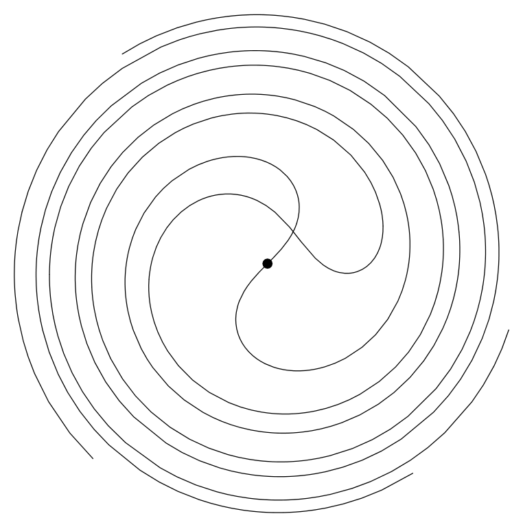
In [8] the boundary value problem for rotating soliton solutions has been discussed. The corresponding local existence result has been generalised to arbitrary Killing fields in [9]. For rotating solitons in the euclidean plane, so called yin-yang curves, a quantity was identified that remains invariant along the curve (see [9]). This invariant allowed to show that yin-yang curves share fundamental geometric properties with geodesic curves. In [9] the corresponding results have been generalised to arbitrary soliton curves on surfaces (see Figure 1).

In addition, it was observed in [9], that translating solitons in the euclidean plane, the so called grim reaper curves, actually are geodesics with respect to a conformally deformed Riemannian metric. Therefore the natural question arose whether soliton curves are (at least locally) always geodesic curves with respect to a modified Riemannian metric. This is not the case. On a surface \((M,g)\), the solutions of (1.1) are immersed curves on \(M\) which may be reparametrised to become geodesics of the Weyl connection \(\nabla_{g,\mathbf{X}}\) given by \[(\mathbf{Y}_1,\mathbf{Y}_2)\mapsto (D_g)_{\mathbf{Y}_1} \mathbf{Y}_2-g(\mathbf{Y}_1,\mathbf{Y}_2)\mathbf{X}+g(\mathbf{X},\mathbf{Y}_1)\mathbf{Y}_2+g(\mathbf{X},\mathbf{Y}_2)\mathbf{Y}_1,\] where we have written \(D_g\) for the Levi-Civita connection of \(g\). The equation (1.1) is parametrisation invariant and thus its solutions are naturally interpreted as the geodesics of a projective structure on \(M\). Recall that a projective structure is an equivalence class of affine torsion-free connections, where two such connections are said to be equivalent if they have the same geodesics up to parametrisation. Recently in [4], Bryant, Dunajski and Eastwood determined the necessary and sufficient local conditions for an affine torsion-free connection to be projectively equivalent to a Levi-Civita connection. Applying their results¹ it follows that the Weyl connection whose geodesics are the yin-yang curves is not projectively equivalent to a Levi-Civita connection. However Jürgen Moser conjectured² that soliton curves can at least locally be interpreted as geodesics of a Finsler metric. Recent results about Finsler metrisability of path geometries by Álvarez Paiva and Berck [1] show that this is indeed the case. Of course, one can ask analogue questions also for higher dimensional solitons. Before we do that, we generalise the notion of soliton solutions slightly.

Note that the \(\mathbf{0}\)-pseudosoliton hypersurfaces are the minimal hypersurfaces of \((M,g)\). It was observed in [13] (see also [7]) that solitons with respect to gradient vector fields correspond to minimal hypersurfaces. However it was left open if such a correspondence holds when the vector field is not the gradient of a smooth function. In this short article we provide an answer using the framework of Monge-Ampère differential systems.

In §2 we will associate to the \(\mathbf{X}\)-pseudosoliton hypersurface equation on \((M,g)\) a Monge-Ampère system on the unit tangent bundle of \(M\) whose Legendre integral manifolds, which satisfy a natural transversality condition, locally correspond to \(\mathbf{X}\)-pseudosoliton hypersurfaces on \(M\). We then show that for a gradient vector field \(\mathbf{X}=\nabla_g u\) on \(M\), the \(\mathbf{X}\)-pseudosoliton M.A.S. is equivalent to the minimal hypersurface M.A.S. on \((M,e^{-2u}g)\). This was already shown in [13], albeit expressed in different language. We complete the picture by proving the

Theorem 1.2 is wrong for \(n=1\), i.e. the case of curves on surfaces. We provide counterexamples and comment on the necessary and sufficient conditions for \(\mathbf{X}\) in the surface case. Theorem 1.2 provides an answer to the equivalence problem for specific M.A.S. in arbitrary dimension \(n+1\geqslant 3\). The equivalence problem for general M.A.S. has been studied for \(5\)-dimensional contact manifolds in [5] and in various low dimensions in [11].

Throughout the article manifolds are assumed to be connected and smoothness, i.e. infinite differentiability is assumed.

Acknowledgements

The second author is grateful to Robert Bryant for helpful discussions. Research for this article was carried out while the authors were supported by the Swiss National Science Foundation, the first author by the grant 200020-124668 and the second by the postdoctoral fellowship PBFRP2-133545.

2 Equivalence of the soliton and minimal hypersurface equation

2.1 Monge-Ampère systems

Let \(N\) be a \((2n+1)\)-dimensional manifold carrying a contact structure, meaning a maximally nonintegrable codimension 1 subbundle \(\mathrm{D}\subset TN\) which we assume to be given by the kernel of a globally defined contact form \(\theta\). Recall that a \(n\)-dimensional submanifold \(f: \Sigma \to N\) which satisfies \(f^*\theta=0\) is called a Legendre submanifold of \((N,\mathrm{D})\). A Monge-Ampère differential system on \((N,\mathrm{D})\) is a differential ideal \(\mathcal{M} \subset \mathcal{A}^*(N)\) in the exterior algebra of differential forms on \(N\) given by \[\mathcal{M}=\left\{\theta,\mathrm{d}\theta,\varphi\right\},\] where \(\varphi \in \mathcal{A}^n(N)\) is a \(n\)-form.³ The brackets \(\{\;\}\) denote the algebraic span of the elements within, i.e. the elements of \(\mathcal{M}\) may be written as \[\alpha\wedge\theta+\beta\wedge \mathrm{d}\theta+\gamma\wedge \varphi,\] where \(\alpha,\beta,\gamma\) are differential forms on \(N\). Note that \(\mathcal{M}\) is indeed a differential ideal since \(\mathrm{d}\varphi\) lies in the contact ideal \(\mathcal{C}=\left\{\theta,\mathrm{d}\theta\right\}\), cf. [5]. A Legendre submanifold of \((N,\mathrm{D})\) which pulls-back to \(0\) the \(n\)-form \(\varphi\) as well will be called a Legendre integral manifold of \(\mathcal{M}\). Two Monge-Ampère systems \((N,\mathcal{M})\) and \((\bar{N},\bar{\mathcal{M}})\) are called equivalent if there exists a diffeomorphism \(\psi : N \to \bar{N}\) identifying the two ideals. Note that this implies that \(\psi\) is a contact diffeomorphism.

2.2 Minimal hypersurfaces via frames

In order to fix notation we review the description of minimal hypersurfaces using moving frames. For \(n \geqslant 1\), let \((M,g)\) be an oriented Riemannian \((n+1)\)-manifold, \(\pi : F \to M\) its right principal \(SO(n+1)\)-bundle of positively oriented orthonormal frames and \(\tau : U \to M\) its (sphere) bundle of unit tangent vectors. Write the elements of \(F\) as \((p,e_0,\ldots,e_n)\) where \(p \in M\) and \(e_0,\ldots,e_n\) is a positively oriented \(g\)-orthonormal basis of \(T_pM\). The Lie group \(SO(n+1)\) acts smoothly from the right by \[(p,e_0,\ldots,e_n)\cdot r=\left(p,\sum_{i=0}^n e_i r_{i0},\dots, \sum_{i=0}^n e_i r_{in}\right),\] where \(r_{ik}\) for \(i,k=0,\ldots,n\) denote the entries of the matrix \(r\). The map \(\nu : F \to U\), given by \((p,e_0,\ldots,e_n) \mapsto (p,e_0)\) is a smooth surjection whose fibres are the \(SO(n)\)-orbits and thus makes \(F\) together with its right action into a \(SO(n)\)-bundle over \(U\). Here we embed \(SO(n)\) as the Lie subgroup of \(SO(n+1)\) given by \[\left\{\left(\begin{array}{cc} 1 & 0 \\ 0 & r \end{array}\right) \in SO(n+1), r \in SO(n) \right\}.\] Let \(\omega_i \in \mathcal{A}^1(F)\) denote the tautological forms of \(F\) given by \[\left(\omega_i\right)_{(p,e_0,\ldots,e_n)}(\xi)=g_p\left(e_i,\pi^{\prime}(\xi)\right),\] and \(\omega_{ik} \in \mathcal{A}^1(F)\) the Levi-Civita connection forms which satisfy \(\omega_{ik}+\omega_{ki}=0\). The dual vector fields to the coframing \(\left(\omega_i,\omega_{ik}\right), i < k\), will be denoted by \(\left(\mathbf{W}_i,\mathbf{W}_{ik}\right)\). Recall that we have the structure equations \[ \begin{aligned} \mathrm{d}\omega_i+\sum_{k=0}^n\omega_{ik}\wedge\omega_k&=0,\\ \mathrm{d}\omega_{ik}+\sum_{l=0}^n\omega_{il}\wedge\omega_{lk}&=\Omega_{ik}, \end{aligned}\](2.1) where \(\Omega_{ik} \in \mathcal{A}^2(F)\) are the curvature forms. Denote by \(\hat{\omega}_i\) the wedge product of the forms \(\omega_1,\ldots \omega_n\), with the \(i\)-th form omitted \[\hat{\omega}_i=\omega_1\wedge\cdots\wedge\omega_{i-1}\wedge\omega_{i+1}\wedge \cdots \wedge \omega_n.\] For \(n=1\) set \(\hat{\omega}_1\equiv1.\) Note that the forms \[\begin{aligned} \theta&=\omega_0,\\ \omega&=\omega_1\wedge \cdots \wedge \omega_n,\\ \mu&=-\frac{1}{n}\sum_{i=1}^n (-1)^{i-1}\omega_{0i} \wedge \hat{\omega}_i,\\ \end{aligned}\] are \(\nu\)-basic, i.e. pullbacks of forms on \(U\) which, by abuse of language, will also be denoted by \(\theta,\omega,\mu\). Since \[ \mathrm{d}\omega_0=-\sum_{k=1}^n\omega_{0k}\wedge \omega_k\](2.2) the \(1\)-form \(\theta\) is a contact form. Note also that \[ \mathrm{d}\omega+(-1)^{n-1}\,n\,\mu\wedge\theta=0.\](2.3) The geometric significance of these forms is the following: Suppose \(f : \Sigma \to M\) is an oriented hypersurface and \(\mathcal{G}_f : \Sigma \to U\) its orientation compatible Gauss lift. In other words the value of \(\mathcal{G}_f\) at \(p \in \Sigma\) is the unique unit vector at \(f(p)\) which is \(g\)-orthogonal to \(f^{\prime}(T_p\Sigma)\) and together with a positively oriented basis of \(T_p\Sigma\) induces the positive orientation of \(T_{f(p)}M\). By construction we have \[ \mathcal{G}_f^*\theta=0\](2.4) and simple computations show that \[ \mathcal{G}_f^*\omega=\omega_{f^*g},\](2.5) where \(\omega_{f^*g}\) denotes the Riemannian volume form on \(\Sigma\) induced by \(f^*g\). Suppose \(\tilde{f} : V \subset \Sigma\to F\) is a local framing covering \(\mathcal{G}_f\) and \(f\). Then pulling back (2.4) and using (2.2) gives \[\sum_{k=1}^n\tilde{f}^*{\omega_{0k}}\wedge \tilde{f}^*{\omega_k}=0.\] The independence (2.5) implies that the forms \(\varepsilon_i=\tilde{f}^*\omega_i\) are linearly independent and thus Cartan’s lemma yields the existence of functions \(h_{ik} : V \to \mathbb{R}\), symmetric in the indices \(i,k\), such that \[\tilde{f}^*\omega_{0i}=\sum_{k=1}^n h_{ik} \varepsilon_k.\] In particular we have \[ \mathcal{G}_f^*\mu=-H \varepsilon_1\wedge\cdots\wedge\varepsilon_n,\](2.6) where \(H=\frac{1}{n}\sum_{i=1}^n h_{ii}\) is the mean curvature of the hypersurface \(f : \Sigma \to M\). Conversely if \(\mathcal{G} : N \to U\) is an orientable \(n\)-submanifold with \(\mathcal{G}^*\theta=0\) and \(\mathcal{G}^*\omega \neq 0\), then \(\tau \circ \mathcal{G} : N \to M\) is an immersion. Shrinking \(N\) if necessary we can assume that \(f=\tau \circ \mathcal{G} : N \to M\) is a hypersurface which can be oriented in such a way that its Gauss lift agrees with \(\mathcal{G}\). Thus the Legendre integral manifolds \(\mathcal{G} : \Sigma \to U\) of the M.A.S. \(\mathcal{M}_g\) on \(U\) given by \[\mathcal{M}_g=\left\{\theta,\mathrm{d}\theta,\mu\right\}\] which satisfy the transversality conditions \(\mathcal{G}^*\omega\neq0\) locally correspond to minimal hypersurfaces on \((M,g)\).

2.3 \(\mathbf{X}\)-pseudosoliton hypersurfaces via frames

Given a vector field \(\mathbf{X}\) on \(M\) define the functions \(X_i : F \to \mathbb{R}\) by \[ (p,e_0,\ldots,e_n) \mapsto g_p(\mathbf{X}(p),e_i).\](2.7) Of course \(X_0\) is the \(\nu\)-pullback of a function on \(U\) which will be denoted by \(X\). Using (1.1) and (2.6) it follows that an oriented hypersurface \(f : \Sigma \to M\) is a \(\mathbf{X}\)-pseudosoliton hypersurface if and only if \[\mathcal{G}_f^*\left(\mu-X\omega\right)=0.\] Thus the Legendre integral manifolds \(\mathcal{G} : \Sigma \to U\) of the M.A.S. \(\mathcal{M}_{g,\mathbf{X}}\) on \(U\) given by \[\mathcal{M}_{g,\mathbf{X}}=\left\{\theta,\mathrm{d}\theta,\mu-X\omega\right\}\] which satisfy the transversality conditions \(\mathcal{G}^*\omega\neq0\) locally correspond to \(\mathbf{X}\)-pseudosoliton hypersurfaces on \((M,g)\). Now suppose \(\mathbf{X}\) is a gradient vector field \(\mathbf{X}=\nabla_g u\) for some smooth function \(u : M \to \mathbb{R}\). Let \(\bar{g}=e^{-2u}g\), \(\bar{\pi} : \bar{F} \to M\) denote the bundle of positively oriented \(\bar{g}\)-orthonormal frames with canonical coframing \(\bar{\omega}_i, \bar{\omega}_{ik}\) and \(\tilde{\psi} : F \to \bar{F}\) the map which scales a \(\bar{g}\)-orthonormal frame by \(e^{u}\). Then by definition \[ \tilde{\psi}^*\bar{\omega}_i=e^{-u}\omega_i,\](2.8) and the structure equations (2.1) yield \[ \tilde{\psi}^*\bar{\omega}_{ik}=\omega_{ik}+u_k\omega_i-u_i\omega_k,\](2.9) where we expand \(\pi^*\mathrm{d}u=\sum_{k=0}^n u_k \omega_k\) for some smooth functions \(u_k : F \to \mathbb{R}\). Note that \(u_0\) is the \(\nu\)-pullback of the function \(X\). Let \(\bar{\tau} : \bar{U} \to M\) denote the \(\bar{g}\)-unit tangent bundle with canonical forms \(\bar{\mu},\bar{\omega}\) and \(\psi : U \to \bar{U}\) the map which scales a \(g\)-unit vector by \(e^u\). Then (2.8) implies \[\psi^*\bar{\omega}=e^{-nu}\omega,\] thus \(\psi\) is a contact diffeomorphism. Moreover (2.8) and (2.9) yield \[ \begin{aligned} \psi^*\bar{\mu}&=-\frac{e^{-(n-1)u}}{n}\sum_{k=1}^n (-1)^{k-1}\left(\omega_{0k}+u_k\theta-u_0\omega_k\right)\wedge \hat{\omega}_k\\ &=-e^{-(n-1)u}\left(\mu-X\omega+\frac{1}{n}\theta\wedge\left(i_{\nabla_g u}\omega\right)\right)\\ \end{aligned}\](2.10) which can be written as \(\alpha\wedge\theta+\gamma\wedge(\mu-X\omega)\) for some \((n-1)\)-form \(\alpha\) and some smooth real-valued function \(\gamma\) on \(U\). This yields \[\psi^*\mathcal{M}_{e^{-2u}g}=\mathcal{M}_{g,\nabla_{g} u}.\] Summarising we have proved the

2.4 The non-gradient case

Proposition 2.1 raises the question if there still exists a contact equivalence between minimal hypersurfaces and solitons if \(\mathbf{X}\) is not a gradient vector field. We will argue next that this is not possible for \(n \geqslant 2\), so assume in this subsection that \(n\geqslant 2\). Before providing the arguments we recall a result from symplectic linear algebra. Suppose \((V,\Theta)\) is a symplectic vector space of dimension \(2n\), i.e.  \(\Theta \in \Lambda^2(V^*)\) is non-degenerate. If a form \(\beta\) of degree \(s \leqslant p\) satisfies \[ \beta\wedge\Theta^{(n-p)}=0,\](2.11) then \(\beta=0\). This is a corollary of the Lepage decomposition theorem for \(p\)-forms on symplectic vector spaces. (cf. [10]). Of course in our setting the symplectic vector spaces are the fibres of the contact subbundle \(D\) and \(\Theta\) is obtained by restricting \(\mathrm{d}\theta\) to \(D\).

Using this Lemma we can proof Theorem 1.2

2.5 The surface case

Recall that in the case \(n=1\) of a surface \((M,g)\), the solutions of the \(\mathbf{X}\)-pseudosoliton equation (1.1) are immersed curves on \(M\) which may be repa- rametrised to become geodesics of a Weyl connection. In his Ph.D. thesis [12], the second author has constructed a \(10\)-parameter family of Weyl connections on the \(2\)-sphere whose geodesics are the great circles, and thus in particular projectively equivalent to the Levi-Civita connection of the standard spherical metric. Inspection shows that there are Weyl connections in this \(10\)-parameter family whose vector field is not a gradient and thus they provide counterexamples to Theorem 1.2 in the surface case.

This raises the question what the necessary and sufficient conditions for the \(\mathbf{X}\)-pseudosolitons curves are, in order to be the geodesics of a Riemannian metric. In [12] it was also shown that on a surface locally every affine torsion-free connection is projectively equivalent to a Weyl connection. Finding the necessary and sufficient conditions thus comes down to finding the necessary and sufficient conditions for an affine torsion-free connection to be projectively equivalent to a Levi-Civita connection. Therefore the conditions follow by applying the results in [4] and we refer the reader to this source for further details.

References

[1]J. C. Alvarez-Paiva, G. Berck, Finsler surfaces with prescribed geodesics, 2010, arXiv:1002.0243.
[2]S. Angenent, On the formation of singularities in the curve shortening flow, J. Differential Geom.33 (1991), 601–633.
[3]S. B. Angenent, Shrinking doughnuts, in Nonlinear diffusion equations and their equilibrium states, 3 (Gregynog, 1989), Progr. Nonlinear Differential Equations Appl.7, Birkhäuser Boston, Boston, MA, 1992, pp. 21–38.
[4]R. Bryant, M. Dunajski, M. Eastwood, Metrisability of two-dimensional projective structures, J. Differential Geom.83 (2009), 465–499.
[5]R. Bryant, P. Griffiths, D. Grossman, Exterior differential systems and Euler-Lagrange partial differential equations, Chicago Lectures in Mathematics, University of Chicago Press, Chicago, IL, 2003.
[6]J. Clutterbuck, O. C. Schnürer, F. Schulze, Stability of translating solutions to mean curvature flow, Calc. Var. Partial Differential Equations29 (2007), 281–293.
[7]G. Huisken, Asymptotic behavior for singularities of the mean curvature flow, J. Differential Geom.31 (1990), 285–299.
[8]N. Hungerbühler, K. Smoczyk, Soliton solutions for the mean curvature flow, Differential Integral Equations13 (2000), 1321–1345.
[9]N. Hungerbühler, B. Roost, Mean curvature flow solitons, in Analytic aspects of problems in Riemannian geometry: Elliptic PDEs, solitons and computer imaging, Séminaires et Congrès19, Société Mathématique de France, 2009, pp. 129–158.
[10]P. Libermann, C.-M. Marle, Symplectic geometry and analytical mechanics, Mathematics and its Applications35, D. Reidel Publishing Co., Dordrecht, 1987, Translated from the French by Bertram Eugene Schwarzbach.
[11]V. V. Lychagin, V. N. Rubtsov, I. V. Chekalov, A classification of Monge-Ampère equations, Ann. Sci. École Norm. Sup. (4)26 (1993), 281–308.
[12]T. Mettler, On the Weyl metrisability problem for projective surfaces and related topics, Ph.D. thesis, Université de Fribourg, Switzerland, 2010.
[13]K. Smoczyk, A relation between mean curvature flow solitons and minimal submanifolds, Math. Nachr.229 (2001), 175–186.
Since the computations are somewhat complex, they have been carried out using maple. The maple file can be obtained from the authors upon request.↩︎
Stated on the occasion of a seminar talk of the first author at the Institute for Mathematical Research (FIM) at ETH Zürich, March 1999.↩︎
More generally one can define a M.A.S. to be a differential ideal which is only locally generated by a contact ideal and an \(n\)-form. However for our purposes the above definition is sufficient.↩︎